Sound-based Anomaly Detection (SAD) for Folks in a Hurry

Machines of all kinds are used to perform different tasks in the manufacturing industry. Loosely put, they are placed together like lego pieces with each individual block serving a useful purpose as the next. A by-product of running all these machines is the symphony they create, just like musicians in an orchestra, with the operations manager being the conductor. Unlike an orchestra, this is a symphony of engines, turbines, pumps, valves, motors, fans, sliders, and so on. In most cases, all stakeholders would love to always keep this show going — to fatten the bottom line. However, there are limitations to how long the show can stay on. Just like humans, machines do get tired, just a different kind of tiredness. And as you’ve guessed, the show can’t go on without all machines working in their best condition. But how do you ensure maximum showtime (uptime), while reducing the risk of malfunctioning machine parts? One approach is to find the machine that is getting out of tune (based on sound). This is known as anomaly detection.

Anomaly detection is the process of identifying differences, variations, deviations from a norm.

There are various methods of detecting anomalies. Some AI and classical machine learning methods involve a rule-based approach defined by a domain expert. Other robust approaches involve gaining insight from the data without specifying/defining a set of rules. Machine learning/deep learning algorithms that can perform anomaly detection will learn what is considered normal from the dataset. One such common algorithm is the autoencoder.

Autoencoders

Autoencoders are networks designed to learn representations of the input data, called latent representations or codings, without any supervision (unsupervised learning). The objective of autoencoders is to learn to copy their inputs to their outputs by adjusting the network parameters to obtain a good compressed knowledge representation of the input data. Without going into too many details — which can be found here or here — autoencoders are designed such that the codings typically have a much lower dimensionality compared to the input it codes/represents. This is achieved by having a bottleneck in the middle of the network architecture to force the compression of the input data. Although other variants of autoencoders do exist, the variation with a bottleneck (under complete) will be discussed here, as illustrated below.

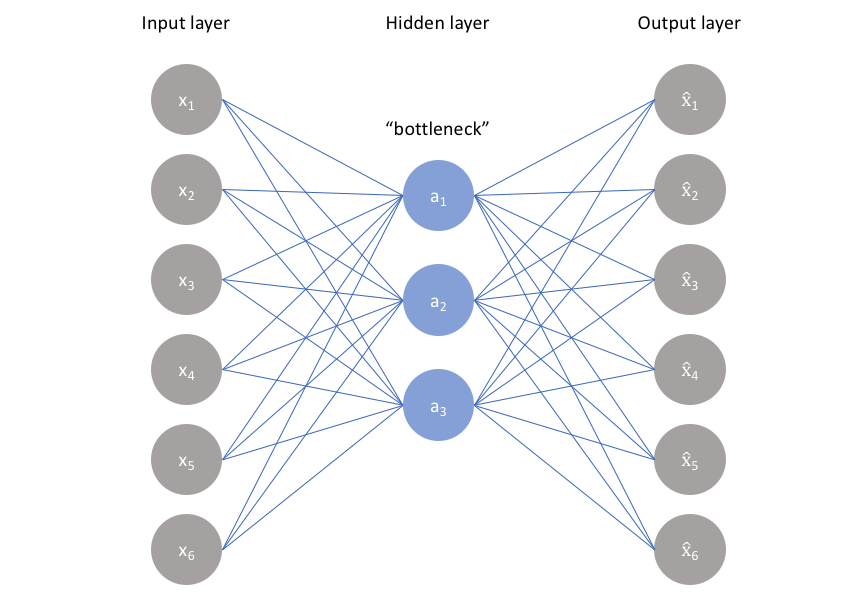
As illustrated above, each output node x-hat is an attempt to reconstruct its respective input node x. The network learns to encode x as a, and decode a to obtain x-hat. The network can be trained by minimizing the reconstruction error, L(x, x-hat), which measures the differences between the original input and the network’s reconstruction (output). This makes the task unsupervised learning disguised as a supervised one. After training the autoencoder, its reconstruction error is expected to be low, for it has successfully learned to reconstruct the input data. Since the autoencoder is trained on only normal data, the reconstruction error of anomalous data is expected to be high, as the autoencoder will fail to reconstruct this anomalous data as well as it would normal data. For us to know what is normal, and what is anomalous, we simply set a threshold (sort of an upper-bound) based on the reconstruction error obtained after training the autoencoder. This means any data with a reconstruction error below the threshold are classified as normal, and data with a reconstruction error above the threshold is classified as an anomaly, turning the inference into a binary classifier.

Note: The network architecture of an autoencoder is not restricted to fully connected layers alone. Other network types such as CNN, RNN, or even combinations of those could be used to build an autoencoder, as long as there is an encoder (that learns and describe latent attributes of the input) and a decoder (that learns to reconstruct the input from the encodings).

SAD with Autoencoders

Here, the sound dataset for malfunctioning industrial machine investigation and inspection (MIMII) is used. More details about the dataset can be obtained from the dataset’s publication. The normal machine sounds from the dataset are split into training, validation, and testing sets. While all the abnormal sounds are used for testing the autoencoder.

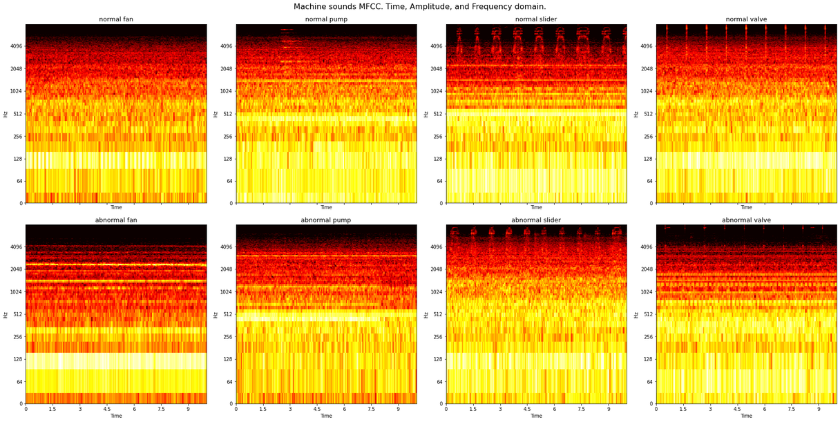
A combination of CNN with fully connected layers is used here as shown in the model summary above. CNN is used as sound data has an image-like representation when converted to a spectrogram, as shown in the diagram below. Refer to this page for more on this. This spectrogram can then be used to train the network just as you would any other image. The diagram below shows a spectrogram of different machine types in normal and abnormal conditions.

After training the model with the normal data set aside for training, reconstruction loss distribution of the model on all the data splits (train, test, and validation) was obtained to visualize the best threshold. The image below shows this loss distribution with various annotated threshold values.

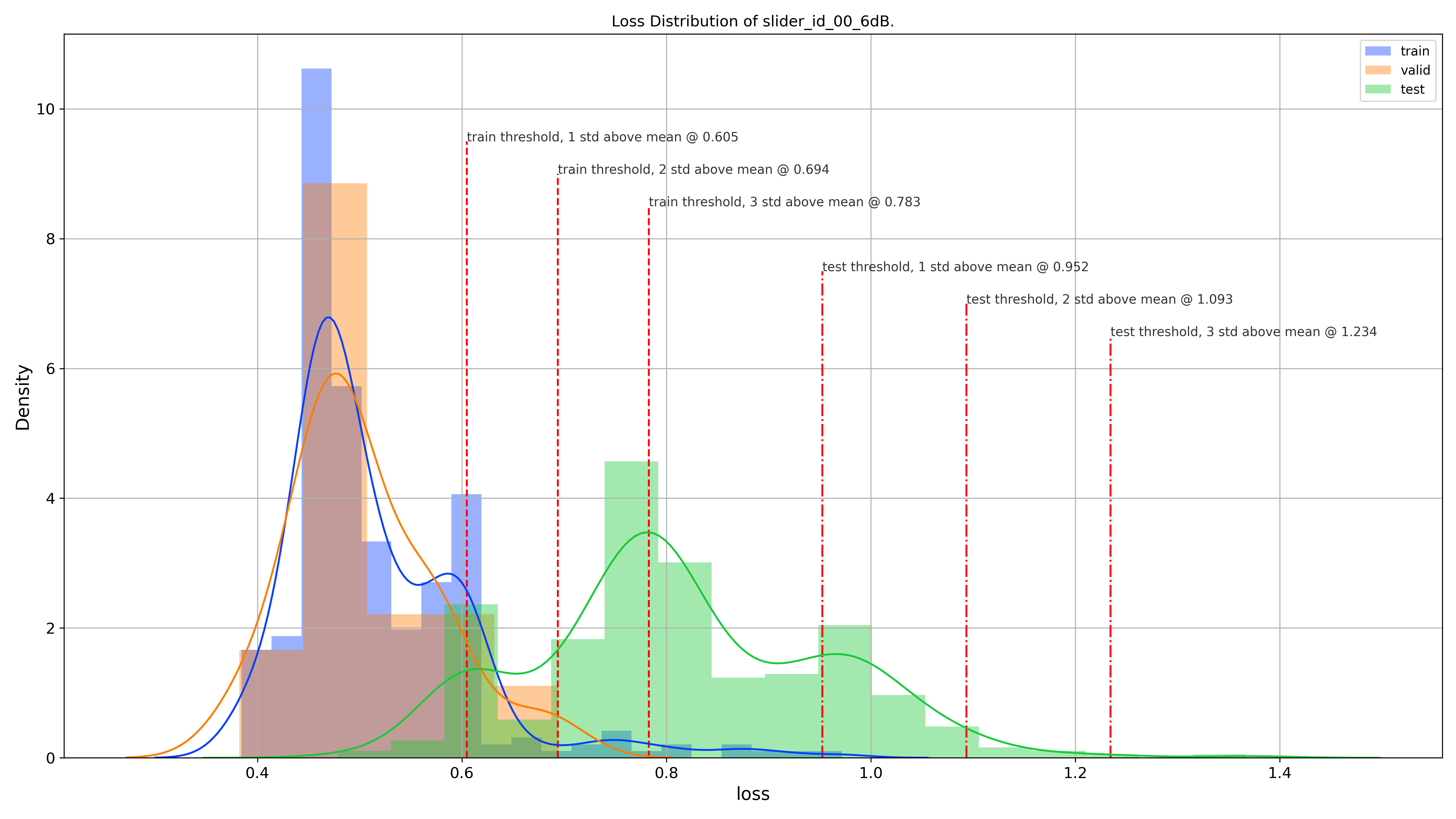
A few observations could be made from this reconstruction loss distribution:

The reconstruction loss distribution of the training data overlaps with that of the validation data
The separation between the reconstruction loss distribution of training/validation data and testing data is very distinct. Meaning, less overlap between normal and abnormal reconstruction loss distribution
There seems to be a point where the reconstruction loss distribution of all data (training, validation, and testing) overlap. This could be contributed by those few normal sound files set aside for testing.

Note: In the real world, it is extremely difficult to have/gather an adequate amount of anomalous data. In some cases, less than 1% of available data are anomalous. This is why unsupervised learning techniques are usually favored for anomaly detection over supervised learning.

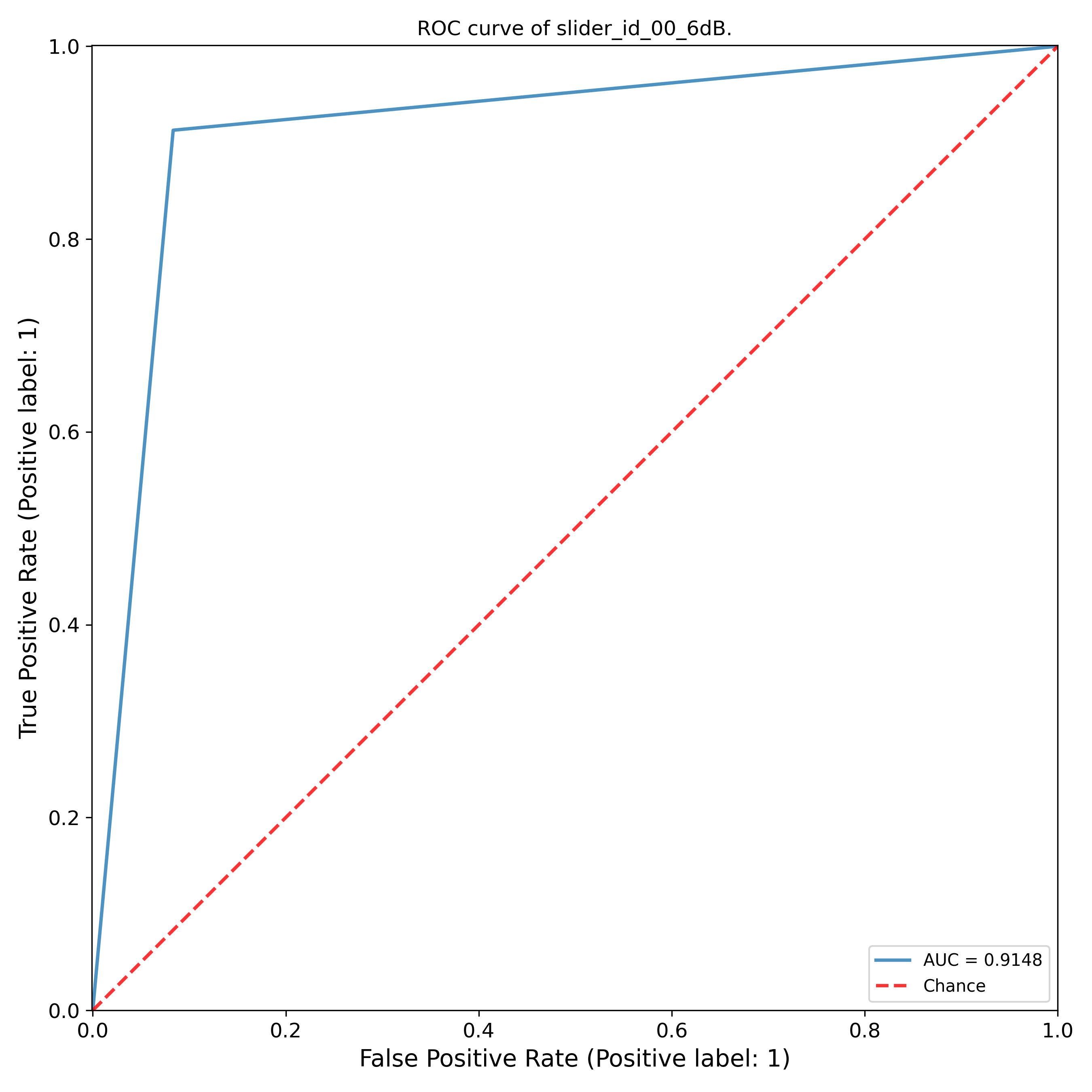
The threshold selected plays a major role in the confusion matrix. Depending on the business needs, higher recall could be much more important than anything else to prevent or reduce false alarms. On the other hand, priority could be placed on maximizing specificity.Below shows the roc curve and the AUC for this model.

Below shows the confusion matrix for a threshold of one standard deviation above the mean of the train loss distribution and the classification report

Conclusion

As you can see, SAD is quite possible by employing autoencoders. Rather than using autoencoders that represent/encodes the data as a single value in the latent space, variational autoencoders could be used as it represents each latent attribute as a probability distribution. Although the result of only one machine at one noise level is reported here, the work was done on all the available machines for all noise levels in the MIMII dataset. You can refer to this repository to play around with the SAD code. Please feel free to contribute to the research and improve the work.